A new generalization of generalized half-normal distribution: properties and regression models

Abstract

In this paper, a new extension of the generalized half-normal distribution is introduced and studied. We assess the performance of the maximum likelihood estimators of the parameters of the new distribution via simulation study. The flexibility of the new model is illustrated by means of four real data sets. A new log-location regression model based on the new distribution is also introduced and studied. It is shown that the new log-location regression model can be useful in the analysis of survival data and provides more realistic fits than other competitive regression models.

Introduction

The generalized half-normal (GHN) distribution has been widely modified and studied in recent years and various authors developed new generalizations of it. Following an idea due to Eugene et al. (2002), Pescim et al. (2017) introduced the beta generalized half-Normal (BGHN) distribution with applications to myelogenous leukemia data. Cordeiro et al. (2012) defined the Kumaraswamy generalized half-normal (KwGHN) distribution for censored data. More recently, Cordeiro et al. (2013) studied some of the mathematical properties of the BGHN distribution proposed by Pescim et al. (2010b). Pescim et al. (2013) proposed the log-linear regression model based on the BGHN distribution, while Ramires et al. (2013) defined the beta generalized half-normal geometric (BGHNG) distribution in order to achieve wider diversity among the density and failure rate functions.

The GHN density function (Cooray and Ananda 2008) with shape parameter λ>0 and scale parameter θ>0 is given (for x>0) by

$$ g(x;\lambda,\theta)=\sqrt{\frac{2}{\pi}}\left(\frac{\lambda}{x}\right) \left(\frac{x}{\theta}\right)^{\lambda}\exp \left[-\frac{1}{2}\left(\frac{x}{\theta}\right)^{2\lambda}\right], $$

(1)

and its cumulative distribution function (cdf) depends on the error function

$$ G(x;\lambda,\theta)=2\Phi \left[\left(\frac{x}{\theta}\right)^{\lambda}\right] -1=erf\left[\frac{\left(\frac{x}{\theta}\right)^{\lambda}}{\sqrt{2}}\right], $$

(2)

where

$$\Phi \left(x\right) =\frac{1}{2}\left[ 1+erf\left(\frac{x}{\sqrt{2}}\right) \right] $$

and

$$erf\left(x\right) =\frac{2}{\sqrt{\pi }}\int_{0}^{x}\exp (-t^{2})dt. $$

The nth moment of the random variable X with cdf (2) is

$$E(X^{n})=\Gamma \left(\frac{n+\lambda }{2\lambda }\right) \frac{\sqrt{\frac{ 2^{\frac{n}{\lambda }}}{\pi }}}{\theta^{-n}}, $$

where Γ(.) is the gamma function. The HN distribution is a sub-model of GHN when λ=1.

The goal of this paper is to propose the first generalization of the generalized half-normal distribution using the Zografos–Balakrishnan Odd Log-Logistic-G (“ZBOLL-G” for short) family of distributions. For an arbitrary baseline cdf G(x), Cordeiro et al. (2015) proposed the probability density function (pdf) f(x) and the cdf F(x) of the ZBOLL-G family of distributions with two additional shape parameters β>0 and α>0 as

$$ f(x;\beta,\alpha,\boldsymbol{\xi})=\frac{\alpha}{\Gamma \left(\beta \right)}\frac{g\left(x;\mathbf{\xi}\right) G^{\alpha -1}(x;\mathbf{\xi })\bar{G}^{\alpha -1}(x;\mathbf{\xi})}{\left[G^{\alpha }(x;\mathbf{\xi})+\bar{G}^{\alpha }(x;\mathbf{\xi})\right]^{2}}\left\{-\log \left[ \frac{\bar{G}^{\alpha}(x;\mathbf{\xi})}{G^{\alpha}(x;\mathbf{\xi })+\bar{G}^{\alpha}(x;\mathbf{\xi})}\right] \right\}^{\beta-1} $$

(3)

and

$$ F(x;\beta,\alpha, \boldsymbol{\xi })=\frac{1}{\Gamma \left(\beta \right) }\gamma\left(\beta,-\log \left[ 1-\frac{G^{\alpha }(x;\mathbf{\xi })}{G^{\alpha}(x;\mathbf{\xi })+\bar{G}^{\alpha }(x;\mathbf{\xi })}\right] \right), \quad x\in \mathfrak{R}, $$

(4)

where ξ denotes the parameter vector of the baseline distribution. We use Eqs. (1), (2) and (3) to obtain the four-parameter ZBOLLGHN pdf (for x>0)

$$ \begin{aligned} f&(x)=\frac{\alpha \sqrt{\frac{2}{\pi}}\left(\frac{\lambda}{x}\right)\left(\frac{x}{\theta}\right)^{\lambda }\exp \left[ -\frac{1}{2}\left(\frac{x}{\theta}\right)^{2\lambda}\right] \left\{2\Phi \left[ \left(\frac{x}{\theta }\right)^{\lambda}\right] -1\right\}^{\alpha-1}\left\{2-2\Phi \left[ \left(\frac{x}{\theta}\right)^{\lambda }\right] \right\}^{\alpha-1}}{\Gamma \left(\beta \right) \left(\left\{ 2\Phi \left[ \left(\frac{x}{\theta }\right)^{\lambda }\right] -1\right\}^{\alpha }+\left\{2-2\Phi \left[ \left(\frac{x}{\theta }\right)^{\lambda}\right] \right\}^{\alpha }\right)^{2}} \\ \times &\left[-\log \left(\frac{\left\{2-2\Phi \left[ \left(\frac{x}{\theta }\right)^{\lambda}\right] \right\}^{\alpha}}{\left\{2\Phi \left[\left(\frac{x}{\theta}\right)^{\lambda}\right] -1\right\}^{\alpha}+\left\{2-2\Phi \left[ \left(\frac{x}{\theta}\right)^{\lambda}\right]\right\}^{\alpha }}\right)\right]^{\beta-1} \quad, \end{aligned} $$

(5)

where α>0, β>0, λ>0 are shape parameters and θ is the scale parameter. The corresponding cdf is given by

$$ F(x)=\frac{1}{\Gamma \left(\beta \right)}\gamma \left[\beta,-\log \left(1-\frac{\left\{2\Phi \left[\left(\frac{x}{\theta}\right)^{\lambda}\right] -1\right\}^{\alpha}}{\left\{2\Phi \left[\left(\frac{x}{\theta} \right)^{\lambda}\right]-1\right\}^{\alpha}+\left\{2-2\Phi\left[\left(\frac{x}{\theta}\right)^{\lambda}\right] \right\}^{\alpha}}\right) \right],\;\; x \geq 0, $$

(6)

where γ(β,z)$=\int \limits _{z}^{\infty }t^{\beta -1}\exp \left (-t\right) dt$ denotes the complementary incomplete gamma function. Henceforth, we denote a random variable X with pdf (5) by X ∼ ZBOLL-GHN(β,α,λ,θ). The sub-models of (5) are given in Table 1.

Table 1 Submodels of ZBOLL-GHN distribution

We investigate the possible hazard rate function (hrf) and pdf shapes of ZBOLL-GHN distribution. Figure 1 displays the pdf shapes of ZBOLL-GHN distribution. Based on the Fig. 1, ZBOLL-GHN pdf has the following shapes: left-skewed, right-skewed, symmetric and bimodal. Figure 2 displays the hrf shapes of ZBOLL-GHN distribution. From Fig. 2, we conclude that the ZBOLL-GHN hrf has the following shapes: increasing, decreasing, upside-down and bathtub.

Fig. 1

The pdf plots of ZBOLL-GHN distribution for selected parameter values

Fig. 2

The hrf plots of ZBOLL-GHN distribution for selected parameter values

Following Cordeiro et al. (2016a), equation (6) can be expressed as

$$F(x)=\sum\limits_{w=0}^{\infty }b_{w}\Pi_{w}\left(x;\lambda,\theta\right), $$

where

$$b_{w}=\frac{1}{\Gamma\left(\beta \right) }\sum\limits_{i,k=0}^{\infty}\sum\limits_{j=0}^{k}\frac{\left(-1\right)^{i+j+k}}{\left(\beta+i-j\right) i!}p_{j,k}a_{w}\left(\beta,\alpha,i,k \right) \binom{k-\beta -i}{k}\binom{k}{j} $$

and Π_w(x;λ,θ)=[G(x;λ,θ)]^w denotes the cdf of the exp-GHN distribution with the power parameter w. The pdf (5) reduces to

$$ f(x)=\sum\limits_{w=0}^{\infty }b_{w+1}\pi_{w+1}\left(x;\lambda,\theta\right), $$

(7)

where π_w+1(x;λ,θ)=(w+1)g(x;λ,θ)[G(x;λ,θ)]^w denotes the pdf of the exp-GHN distribution with the power parameter w+1. For the definitions of p_j,k and a_w(β,α,i,k), please see Cordeiro et al. (2016a). Equation (7) reveals that the density function of X is a linear combination of the exp-GHN densities. Thus, some of the structural properties of the ZBOLL-GHN distribution such as ordinary and incomplete moments and generating function can be obtained from well-established properties of the exp-GHN distribution.

We are motivated to introduce the ZBOLL-GHN distribution since it contains a number of aforementioned known lifetime models as illustrated in Table 1. The new distribution exhibits increasing, decreasing, upside-down as well as bathtub hazard rates as illustrated in Fig. 2. It is shown that the new distribution can be viewed as a mixture of the two-parameter GHN model. It can also be viewed as a suitable model for fitting the left-skewed, right-skewed, symmetric and bimodal data. The ZBOLL-GHN distribution outperforms several of the well-known lifetime distributions with respect to four real data applications as illustrated in “Applications” section. The new log-location regression model based on the ZBOLL-GHN distribution provides better fits than log BGHN, log GHN and log-Weibull models for volatage data set. Based on the residual analysis (martingale and modified deviance residuals) for the new log-location regression model (log ZBOLL-GHN), we conclude that none of the observed values appear as possible outliers. Thus, it is clear that the fitted model is appropriate for the voltage data set.

The rest of the paper is organized as follows. In “Estimation” section, the maximum likelihood method is used to estimate the model parameters. The performance of maximum likelihood estimators of the model parameters are investigated by means of a Monte Carlo simulation study when n is finite. A new log-location regression model as well as residual analysis are presented in “A new log-location regression model” section. Four applications to real data sets illustrate empirically the importance of the new model in “Applications” section. Finally, a summary is provided in “Summary” section.

Estimation

If X follows the ZBOLL-GHN distribution with vector of parameters Ψ=(β,α,λ,θ)^T. The log-likelihood function for a single observation x of X is given by

$$\begin{aligned} \ell (\mathbf{\Psi}) =&\log \left(\alpha\right) +\log \left(\sqrt{\frac{2}{\pi}}\right) +\log \left(\lambda \right) -\log \left(x\right) +\lambda\log \left(x\theta^{-1}\right) -\frac{1}{2}\left(x\theta^{-1}\right)^{2\lambda} \\ +&\left(\alpha -1\right) \log \left(w-1\right) +\left(\alpha-1\right)\log \left(2-w\right) -\log\left[\Gamma\left(\beta \right) \right] \\ &-2\log \left[\left(w-1\right)^{\alpha}+\left(2-w\right)^{\alpha}\right] +\left(\beta -1\right) \log \left[-\log \left(\frac{\left(2-w\right)^{\alpha}}{\left(w-1\right)^{\alpha}+\left(2-w\right)^{\alpha}}\right) \right]. \end{aligned} $$

The components of the unit score vector U=U(Ψ)=(∂β/∂ℓ,∂α/∂ℓ,∂λ/∂ℓ,∂θ/∂ℓ)^T are available if needed. For a random sample x=(x₁,...,x_n)^T of size n from X, the total log-likelihood is

$$\ell_{n}(\mathbf{\Psi})=\sum_{i=0}^{n}\ell^{(i)}(\mathbf{\Psi}), $$

where ℓ⁽ⁱ⁾(Ψ) is the log-likelihood for the i^th observation. The total score function is

$$U_{n}=\sum_{i=0}^{n}U^{(i)}, $$

where U⁽ⁱ⁾ has the form given before. Maximization of ℓ(Ψ) (or ℓ_n(Ψ)) can be easely performed using well-established routines such as the nlm or optim in the R statistical package. Setting these equations equal to zero, U(Ψ)=0, and solving them simultaneously gives the MLE $\widehat {\mathbf {\Psi }}$ of Ψ. These equations cannot be solved analytically and statistical software can be used to evaluate them numerically using iterative techniques such as the Newton-Raphson algorithm.

The parameter estimation procedure of ZBOLL-GHN model can be summarized as follows:

• The optim function of R software is used to minimize the minus log-likelihood function of GHN model by means of the Nelder-Mead (NM) optimization method. There is no need to provide the derivatives of the objective function for NM method.

• The estimated parameters of GHN distribution are used as initial values of the ZBOLL-GHN model. The initial values of the additional parameters α and β are chosen as 1. Note that the ZBOLL-GHN model reduces to GHN model when the parameters α=β=1. Then, the parameter estimation of ZBOLL-GHN model are obtained with the optim function as given in the first step.

• The inverse of estimated Hessian matrix is used to obtain the corresponding standard errors.

Simulation study

In this subsection, the performance of the maximum likelihood estimators of the ZBOLL-GHN parameters are evaluated via a Monte Carlo simulation study with 10,000 replications. The coverage probabilities (CPs), mean square errors (MSES) and the bias of the parameter estimates, estimated average lengths (ALs) are calculated by means of R software. We generate N=10,000 samples of sizes n=50,55,...,500 from the ZBOLL-GHN distribution with α=0.8,β=7,λ=9,θ=4. Let $\left (\widehat {\alpha }, \widehat {\beta },\widehat {\lambda },\widehat {\theta }\right)$ be the MLEs of the new model parameters and $(s_{\widehat {\alpha }},s_{\widehat {\beta }},s_{\widehat {\lambda }},s_{\widehat {\theta }})$ be the standard errors of the MLEs. The estimated biases and MSEs are given by

$$\widehat{Bias}_{\epsilon}(n)=\frac{1}{N}\sum\limits_{i=1}^{N}\left(\hat{\epsilon_{i}}-\epsilon\right) $$

and

$$\widehat{MSE}_{\epsilon}(n)=\frac{1}{N}\sum\limits_{i=1}^{N}\left(\hat{\epsilon_{i}}-\epsilon\right)^{2}, $$

for ε=α,β,λ,θ. The CPs and ALs are given, respectively, by

$${CP}_{\epsilon}(n)=\frac{1}{N}\sum\limits_{i=1}^{N}I\left(\hat{\epsilon_{i}}-1.95996 s_{\hat{\epsilon_{i}}}, \hat{\epsilon_{i}}+1.95996 s_{\hat{\epsilon_{i}}}\right) $$

and

$${AL}_{\epsilon}(n)=\frac{3.919928}{N}\sum\limits_{i=1}^{N}s_{\hat{\epsilon_{i}}}. $$

Figure 3 displays the numerical results for the above measures. We list below the results from these plots:

• ✓ The estimated biases decrease when the sample size n increases,

  Fig. 3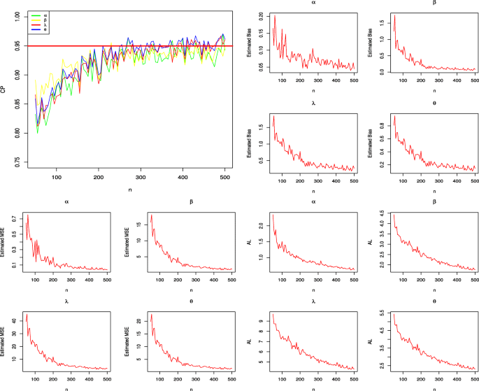

  

  Estimated CPs, biases, MSEs and ALs for the selected parameter values

• ✓ The estimated MSEs decay toward zero as n increases,

• ✓ The CPs are near 0.95 and approach the nominal value when the sample size n increases,

• ✓ The ALs decrease for all parameters when the sample size n increases.

These results reveal the consistency property of the MLEs.

A new log-location regression model

Let X denote a random variable following the ZBOLL-GHN distribution (5) and let Y=log(X). The density function of Y (for $y\in \mathfrak {R}$) and replacing μ= log(θ), $\sigma =\sqrt {2}/{2\lambda }$ can be expressed as

$$ \begin{aligned} f\left(y\right) =&\frac{\alpha}{{\Gamma\left(\beta \right) \sigma \sqrt{2 \pi}}}\exp \left\{ {\ -\frac{1}{2}\exp \left[ {\left(\frac{{y-\mu}}{\sigma}\right) \sqrt{2}}\right]\!+\left(\frac{{y-\mu}}{\sigma}\right) \frac{\sqrt{2}}{2}} \right\} {\left[ {2\Phi \left[ {\exp \left[ {\left({\frac{{y-\mu}}{\sigma}}\right) \frac{\sqrt{2}}{2}}\right]}\right] -1} \right]^{\alpha -1}} \\ &\times {\left({1-\left[{2\Phi \left[{\exp \left[ {\left({\frac{{y-\mu }}{\sigma }}\right) \frac{\sqrt{2}}{2}}\right]} \right]-1}\right]}\right)^{\alpha -1}} \\ &\times \left[\left[{2\Phi \left[\exp \left[ {\left(\frac{y-\mu}{\sigma}\right)\frac{\sqrt{2}}{2}}\right] \right] -1}\right]^{\alpha}+ \left({1-\left[{2\Phi \left[{\exp \left[{\left({\frac{{y-\mu }}{\sigma }}\right) \frac{\sqrt{2}}{2}}\right]}\right]-1}\right]}\right)^{\alpha}\right]^{-2} \\ &\times {\left\{\ -\log \left[\frac{{\left({1-\left[ {2\Phi \left[ {\exp \left[{\left(\frac{{y-\mu}}{\sigma} \right) \frac{\sqrt{2}}{2}}\right] }\right] -1}\right] }\right)}^{\alpha }}{{{\left[ {2\Phi \left[ {\exp \left[ {\left({\frac{{y-\mu }}{\sigma }}\right) \frac{\sqrt{2}}{2}}\right] }\right] -1}\right]}^{\alpha }}+{{\left({1-\left[ {2\Phi \left[ {\exp \left[{\left({\frac{{y-\mu }}{\sigma }}\right) \frac{\sqrt{2}}{2}}\right] }\right] -1}\right] }\right) }^{\alpha}}}\right]\right\}^{\beta -1},} \end{aligned} $$

(8)

where μ∈ℜ is the location parameter, σ>0 is the scale parameter and α>0 and β>0 are the shape parameters. We refer to Eq. (8) as the pdf of LZBOLL-GHN distribution, say Y∼LZBOLL-GHN(α,β,μ,σ). The survival function corresponding to (8) is given by

$$ S\left(y\right) =1-\frac{1}{{\Gamma \left(\beta \right)}}\gamma\!\left(\! {\beta,-\log \left[ {1-\frac{{{{\left[ {2\Phi \left[ {\exp \left[ {\left({\frac{{y-\mu}}{\sigma}}\right) \frac{\sqrt{2}}{2}}\right] }\right]-1}\right] }^{\alpha }}}}{{{{\left[ {2\Phi \left[ {\exp \left[{\left({\frac{{y-\mu}}{\sigma }}\right) \frac{\sqrt{2}}{2}}\right] }\right] -1}\right] }^{\alpha}}+{{\left({1-\left[{2\Phi \left[ {\exp \left[{\left({\frac{{y-\mu }}{\sigma }}\right) \frac{\sqrt{2}}{2}}\right]}\right]-1}\right] }\right)}^{\alpha}}}}}\right] }\right) $$

(9)

The hrf is simply h(y)=f(y)/S(y). The standardized random variable Z=(Y−μ)/σ has density function

$$ \begin{aligned} f(z) =&\frac{\alpha}{\Gamma \left(\beta \right) \sqrt{2\pi}}\exp \left\{ -\frac{1}{2}\exp \left[ {\left(z\right) \sqrt{2}}\right] +\left({\frac{{y-\mu }}{\sigma }}\right) \frac{\sqrt{2}}{2}\right\} {\left[{2\Phi\left[ {\exp \left[{\left(z\right) \frac{\sqrt{2}}{2}}\right]}\right]-1}\right]^{\alpha-1}} \\ &\times {\left({1-\left[ {2\Phi \left[{\exp \left[{\left(z\right) \frac{\sqrt{2}}{2}}\right]}\right]-1}\right]} \right)^{\alpha-1}} \\ &\times {\left[ {\left[{2\Phi \left[{\exp \left[{\left(z\right) \frac{\sqrt{2}}{2}}\right]}\right]-1}\right] }^{\alpha }+{{\left({1-\left[ {2\Phi\left[{\exp \left[{\left(z\right) \frac{\sqrt{2}}{2}}\right]}\right]-1}\right] }\right)}^{\alpha}}\right]^{-2}} \\ &\times\left\{ {\-\log \left[{\frac{{{{\left({1-\left[ {2\Phi \left[{\exp \left[{\left(z\right)\frac{\sqrt{2}}{2}} \right]}\right]-1}\right]}\right)}^{\alpha}}}}{{{{\left[ {2\Phi \left[{\exp \left[ {\left(z\right)\frac{\sqrt{2}}{2}} \right]}\right]-1}\right]}^{\alpha}}+{{\left({1-\left[{2\Phi \left[{\exp \left[{\left(z\right) \frac{\sqrt{2}}{2}} \right]}\right]-1}\right]}\right)}^{\alpha}}}}}\right]}\right\}^{\beta -1}. \end{aligned} $$

(10)

Figure 4 provides some plots of the density function (8) for selected parameter values. They reveal that this distribution is a good candidate to model left skewed and symmetric data sets.

Fig. 4

Plots of the LZBOLL-GHN density function for selected parameter values

Based on the LZBOLL-GHN density, we propose a linear location-scale regression model linking the response variable y_i and the explanatory variable vector $\mathbf {v}_{i}^{\intercal }=(v_{i1},\ldots,v_{ip})$ given by

$$ y_{i} = \mathbf{v}_{i}^{\intercal} {\text{\boldmath \(\beta\)}} + \sigma z_{i}, \; i=1, \ldots,n, $$

(11)

where the random error z_i has density function (10), $\boldmath {\beta }=(\beta _{1},\ldots,\beta _{p})^{\intercal }$, and σ>0, α>0 and β>0 are unknown parameters. The parameter $\mu _{i}=\mathbf {v}_{i}^{\intercal } \boldmath {\beta }$ is the location of y_i. The location parameter vector ${\boldmath {\mu }}=(\mu _{1},\ldots,\mu _{n})^{\intercal }$ is represented by a linear model μ=Vβ, where $\mathbf {V}=(\mathbf {v}_{1},\ldots,\mathbf {v}_{n})^{\intercal }$ is a known model matrix.

The LZBOLL-GHN model (11) provides new opportunities for modeling several types of data sets. This model contains two important regression models as its sub-models: (i) for β=1, the LZBOLL-GHN model reduces to log-OLL-GHN regression model introduced by Pescim et al. (2017); (ii) for α=β=1, the LZBOLL-GHN model reduces to log-GHN regression model.

Let F and C be the sets of individuals for which y_i is the log-lifetime or log-censoring, respectively. Assume that the observed lifetimes and censoring times are independent. The log-likelihood function for the vector of parameters $\Theta =(\alpha,\beta,\sigma,\boldmath {\beta }^{\intercal })^{\intercal }$ from model (11) is given by $l(\Theta)=\sum \limits _{i \in F}l_{i}(\Theta)+\sum \limits _{i \in C}l_{i}^{(c)}(\Theta)$, where l_i(Θ)= log[f(y_i)], $l_{i}^{(c)}(\Theta)=\log [S(y_{i})]$. The f(y_i) and S(y_i) are defined in(8) and (9), respectively. The total log-likelihood function for Θ is given by

$$ \begin{aligned} \ell \left(\Theta \right) =& r\log \left(\frac{\alpha }{\Gamma \left(\beta \right)\sigma \sqrt{2\pi}}\right) -\frac{1}{2}\sum\limits_{i\in F}\exp\left({{z_{i}}\sqrt{2}}\right) +\frac{\sqrt{2}}{2}\sum\limits_{i\in F}{ z_{i}} \\ & +(\alpha-1) \sum\limits_{i\in F}\log \left[u_{i}-1\right] + (\alpha-1) \sum\limits_{i\in F}\log \left(2-u_{i}\right)-2\sum\limits_{i\in F}\log \left[\left[u_{i}-1\right]^{\alpha}+\left(2-u_{i}\right)^{\alpha}\right] \\ & +(\beta -1) \sum\limits_{i\in F}\log \left\{-\log \left[\frac{\left(2-u_{i}\right)^{\alpha}}{\left[u_{i}-1\right]^{\alpha} + \left(2-u_{i}\right)^{\alpha}}\right]\right\}\\ & +\sum\limits_{i\in C}\log \left\{1-\frac{1}{\Gamma(\beta)}\gamma \left(\beta, -\log\left[1-\frac{\left[u_{i}-1\right]^{\alpha}}{\left[u_{i}-1\right]^{\alpha}+\left(2-u_{i}\right)^{\alpha}}\right] \right) \right\}, \end{aligned} $$

(12)

where ${u_{i}}=2\Phi [\exp (z_{i}\sqrt {2}/2)]$, z_i=(y_i−μ_i)/σ, and r is the number of uncensored observations (failures). The MLE $\widehat {\Theta }$ of the vector of unknown parameters can be evaluated by maximizing the log-likelihood (12). The R software is used to estimate unknown parameters of LZBOLL-GHN regression model

The likelihood ratio (LR) statistic can be used for comparing some sub-models of LZBOLL-GHN regression model. For example, the LR statistic can be used to discriminate between the LZBOLL-GHN and LGHN regression models since they are nested models, or equivalently to test H₀:α=β=1. The LR statistic reduces to $w=2\left [\ell (\hat {\alpha },\hat {\beta },\hat {\sigma },\boldsymbol {\hat {\beta }})-\ell (1,1,\tilde {\sigma },\boldsymbol {\tilde {\beta }})\right ]$, where $\left (\hat {\alpha },\hat {\beta },\hat {\sigma },\boldsymbol {\hat {\beta }}\right)$ are the unrestricted MLEs and $(1,1,\tilde {\sigma },\boldsymbol {\tilde {\beta }})$ are the restricted estimates under H₀. The statistic w is asymptotically (as n→∞) distributed as $\chi _{k}^{2}$, where k is difference of two parameter vectors of nested models. For example, take k=2 for the above hypothesis test.

Residual analysis

Residual analysis has critical role to check the adequacy of the fitted model. In order to analyze departures from error assumption, two types of residuals are considered: martingale and modified deviance residuals.

Martingale residual

The martingale residuals is defined in counting process and takes values between +1 and −∞ (see for details, Fleming and Harrington (1994)). The martingale residuals for LZBOLL-GHN model is,

$$ r_{M_{i}} = \left\{ \begin{array}{l} 1 + \log \left\{1-\frac{1}{\Gamma(\beta)}\gamma \left(\beta,-\log \left[1-\frac{\left[u_{i}-1\right]^{\alpha}} {\left[u_{i}-1\right]^{\alpha}+\left(2-u_{i}\right)^{\alpha}}\right]\right)\right\} \;\;\text{if} \;\; i \in F, \\ \log \left\{1-\frac{1}{\Gamma(\beta)}\gamma \left(\beta,-\log \left[1-\frac{\left[u_{i}-1 \right]^{\alpha}}{\left[u_{i}-1\right]^{\alpha}+\left(2-u_{i}\right)^{\alpha}}\right]\right)\right\} \;\; \text{if} \;\; i \in C, \end{array}\right. $$

(13)

where $u_{i}=2\Phi \left [\exp \left (z_{i}\sqrt {2}/2\right)\right ]$ and z_i=(y_i−μ_i)/σ.

Modified deviance residual

The main drawback of martingale residual is that when the fitted model is correct, it is not symmetrically distributed about zero. To overcome this problem, modified deviance residual was proposed by Therneau et al. (1990). The modified deviance residual for LZBOLL-GHN model is,

$$ r_{D_{i}} = \left\{ \begin{array}{l} sign\left(\hat{r}_{M_{i}}\right)\left\{ -2\left[ \begin{array}{l} \left(1 +\log \left\{1-\frac{1}{\Gamma (\beta)}\gamma\left(\beta,-\log \left[1-\frac{\left[u_{i}-1\right]^{\alpha}} {\left[u_{i}-1\right]^{\alpha}+\left(2-u_{i}\right)^{\alpha}} \right]\right)\right\}\right)\\ +\log\left(-\log\left\{1-\frac{1}{\Gamma(\beta)}\gamma \left(\beta,-\log \left[1-\frac{\left[u_{i}-1\right]^{\alpha}} {\left[u_{i}-1\right]^{\alpha}+\left(2-u_{i}\right)^{\alpha}}\right]\right)\right\}\right) \end{array} \right] \right\}^{\frac{1}{2}}\mathrm{\ if }\,\,\ i \in F, \\ sign\left(\hat{r}_{M_{i}}\right)\left\{ -2\left[1+\log\left\{1-\frac{1}{\Gamma(\beta)}\gamma \left(\beta,-\log\left[1- \frac{\left[u_{i}-1\right]^{\alpha}}{\left[u_{i}-1\right]^{\alpha}+\left(2-u_{i}\right)^{\alpha}}\right]\right)\right\} \right]\right\}^{\frac{1}{2}} \;\; \text{if} \;\; i\in C, \end{array}\right. $$

(14)

where $\hat r_{M_{i}}$ is the martingale residual.

Applications

In this section, four real data sets are used to compare ZBOLL-GHN model with its sub-models and beta-GHN model introduced by Pescim et al. (2013). The first three data sets are used to demonstrate the univariate data fitting performance of ZBOLL-GHN distribution. The fourth data set is used to investigate the usefulness of the proposed distribution in survival analysis. The optim function is used to estimate the unknown model parameters. The MLEs and corresponding standard errors, estimated −ℓ, Kolmogorov-Smirnov (K-S) statistic and corresponding p-value, Cramér-von Mises (W*), Anderson-Darling (A*) statistics and Akaike Information Criteria (AIC) are reported in Tables 2, 4 and 6. The lower the values of these criteria show the better fitted model on the data sets. The histograms with fitted pdfs are provided for visual comparison of the fitted distribution functions. Moreover, fitted hrfs and P-P plots of the best fitted models are displayed in Figs. 5, 7 and 9.

Fig. 5

a Fitted densities of models and b fitted hrf and P-P plot of the ZBOLL-GHN model for first set

Table 2 MLEs and their SEs of the fitted models and goodness-of-fit statistics for first data set

Lifetime of device data

The first data set is given by Sylwia (2007) on the lifetime of a certain device. Table 2 shows the estimated parameters and their standard errors, −ℓ, A*, W*, K-S and its corresponding p-value and AIC values. Based on the figures in Table 2, it is clear that ZBOLL-GHN model provides the best fit for this data set. Figure 5a displays the estimated pdfs of the fitted models. Figure 5b displays the P-P plot of ZBOLL-GHN distribution and its fitted hrf. Figure 5 shows that ZBOLL-GHN distribution provides superior fit to the left-skewed data set.

Table 3 shows the LR statistics and the corresponding p-values for the first data set. From Table 3, the computed p-values are smaller than 0.05, so the null hypotheses are rejected for all sub-models. We conclude that the ZBOLL-GHN model fits the first data better than its sub-models according to the LR test results.

Table 3 The LR test results for first data set

In addition, the profile log-likelihood functions of the ZBOLL-GHN distribution are plotted in Fig. 6. These plots reveal that the likelihood functions of the ZBOLL-GHN distribution have solutions that are maximizers.

Fig. 6

The profile log-likelihood plots of ZBOLL-GHN for lifetime of a certain device data

Failure times of wind-shield data

The second data set represents the failure times for a particular wind-shield model including 85 observations that are classified as failed times of wind-shields (Murthy et al. 2004). Table 4 shows the estimated parameters and their standard errors, −ℓ and AIC values. Based on the figures in Table 4, ZBOLL-GHN distribution provides the best fit among others. Figure 7a displays the histogram with fitted pdfs and Fig. 7b displays the fitted hrf and P-P plot of ZBOLL-GHN distribution. These figures reveal that ZBOLL-GHN model provides superior fit to the second data set.

Fig. 7

a Fitted densities of the models and b fitted hrf and P-P plot of the ZBOLL-GHN model for second data set

Table 4 MLEs and their SEs of the fitted models and goodness-of-fit statistics for second data set

Table 5 shows the LR statistics and the corresponding p-values for the second data set. From Table 5, the computed p-values are smaller than 0.05, so the null hypotheses are rejected for all sub-models. We conclude that the ZBOLL-GHN model fits the first data better than its sub-models according to the LR test results.

Table 5 The LR test results for second data set

The profile log-likelihood functions of the ZBOLL-GHN distribution are plotted but not included here. These plots reveal that the likelihood functions of the ZBOLL-GHN distribution have solutions that are maximizers.

Strengths of glass fibres data

The third data set obtained from Smith and Naylor (1987) represents the strengths of 1.5 cm glass fibres, measured at the National Physical Laboratory, England. Unfortunately, the units of measurement are not given in the paper. This data set have been analyzed recently with the beta generalized exponential distribution, which was introduced and studied by Barreto-Souza et al. (2010). Table 6 shows the estimated parameters and their standard errors, −ℓ and AIC values. Based on the figures in Table 6, ZBOLL-GHN distribution provides the best fit among others. Figure 8a displays the histogram with fitted pdfs and Fig. 8b displays the fitted hrf and P-P plot of ZBOLL-GHN distribution. These figures reveal that ZBOLL-GHN model provides superior fit to the third data set.

Table 6 MLEs and their SEs of the fitted models and goodness-of-fit statistics for third data set

Fig. 8

a Fitted densities of the models and b fitted hrf and P-P plot of the ZBOLL-GHN model for third data set

Table 7 shows the LR statistics and the corresponding p-values for the third data set. From Table 7, the computed p-values are smaller than 0.05, so the null hypotheses are rejected for all sub-models. We conclude that the ZBOLL-GHN model fits the first data better than its sub-models according to the LR test results.

Table 7 The LR test results for third data set

The profile log-likelihood functions of the ZBOLL-GHN distribution are plotted but not included here. These plots reveal that the likelihood functions of the ZBOLL-GHN distribution have solutions that are maximizers (Fig. 8).

Voltage data

Lawless (2003) reported an experiment in which specimens of solid epoxy electrical-insulation were studied in an accelerated voltage life test. The sample size is n=60, the percentage of censored observations is 10% and there are three levels of voltage: 52.5, 55.0 and 57.5. The variables involved in the study are: x_i- failure times for epoxy insulation specimens (in min); c_i - censoring indicator (0 =censoring, 1 =lifetime observed); v_i1 - voltage (kV).

The data set was used by Pescim et al. (2013) for illustrating the log-B-GHN (LBGHN) regression model. Pescim et al. (2013) compared the log-B-GHN (LBGHN) regression model with LOLLGHN and log-GHN (LGHN) models. In this section we compare the LZBOLL-GHN regression model with models reported in Pescim et al. (2013). The regression model fitted to the voltage data set is given by

$$ y_{i} = \boldsymbol{\beta_{0}} + \boldsymbol{\beta_{1}}x_{i1} + \sigma z_{i}, $$

(15)

where the random variable y_i follows the LZBOLL-GHN distribution given in (8). The results are presented in Table 8. The MLEs of the model parameters and their SEs and the values of the AIC and BIC statistics are listed in Table 8.

Table 8 MLEs of the parameters to the voltage data for LZBOLL-GHN, LBGHN, LGHN and log-Weibull regression models, the corresponding SEs in second line, p-values in third line and the AIC and BIC statistics

Based on the figures in Table 8, we conclude that the fitted LZBOLL-GHN regression model has the lowest AIC and BIC values. Figure 9 provides the plots of the empirical and estimated survival function for the LZBOLL-GHN regression model. We can conclude from these plots that LZBOLL-GHN regression model provides a good fit to the data.

Fig. 9

Estimated survival function of LZBOLL-GHN regression model and empirical survival for the voltage data considering the voltage levels: x_i1 = 52.5; 55.0 and 57.5

Residual Analysis of LZBOLL-GHN model

Figure 10 displays the index plot of the modified deviance residuals and its Q-Q plot against N(0,1) quantiles. Based on the Figure 10, we conclude that none of the observed values appears as a possible outlier. Thus, it is clear that the fitted model is appropriate for these data set (Fig. 10).

Fig. 10

a Index plot of the modified deviance residual and b Q-Q plot for modified deviance residual

Summary

A new model called Zografos-Balarkishnan odd log-logistic generalized half-normal is introduced and studied. We assess the performance of the maximum likelihood estimators of the parameters of the new distribution with respect to the sample size n. The assessment is based on a graphical simulation study. The flexibility of the new model is illustrated by means of the three real data sets. The new model performs much better than beta generalized half-normal, generalized half-normal, odd log-logistic generalized half-normal and the generalized half-normal models. Additionally, a new log-location regression model based on the new distribution is introduced and studied. The martingale residual and the modified deviance residuals to detect outliers and evaluate the model assumptions are defined. We demonstrate that the new log-location regression model can be very useful in the analysis of real data and provide more realistic fits than other regression models such as the log beta generalized half-normal, the log generalized half-normal and the log-Weibull regression models. The potentiality of the new regression model is illustrated by means of a real data.

References

Aarts, R.M.: Lauricella functions (2000). www.mathworld.com/LauricellaFunctions.html. From MathWorld - A Wolfram Web Resource, created by Eric W. Weisstein.
Barreto-Souza, W., Santos, A.H., Cordeiro, G.M.: The beta generalized exponential distribution. J. Stat. Comput. Simul. 80, 159–172 (2010).
Cooray, K., Ananda, M.M.A.: A generalization of the half-normal distribution with applications to lifetime data. Commun. Stat. Theory Methods. 37, 1323–1337 (2008).
Cordeiro, G.M., Alizadeh, M., Ortega, E.M., Serrano, L.H.V.: The Zografos-Balakrishnan odd log-logistic family of distributions: properties and applications. Hacettepe Res. J. Math. Stat. 45, 1781–1803 (2016a).
Cordeiro, G.M., Alizadeh, M., Pescim, R.R., Ortega, E.M.M.: The odd log-logistic generalized half-normal lifetime distribution: properties and applications. Commun. Stat. Theory Methods. 46, 4195–4214 (2016b).
Cordeiro, G.M., Pescim, R.R., Ortega, E.M.M.: The Kumaraswamy generalized half-normal distribution for skewed positive data. J. Data Sci. 10, 195–224 (2012).
Cordeiro, G.M., Pescim, R.R., Ortega, E.M.M., Demétrio, C.G.B.: The beta generalized half-normal distribution: new properties. J. Probab. Stat. 2013, 1–18 (2013).
Eugene, N., Lee, C., Famoye, F.: Beta-normal distribution and its applications. Commun. Stat. Theory Methods. 31, 497–512 (2002).
Exton, H.: Handbook of hypergeometric integrals: theory, applications, tables, computer programs. Halsted Press, New York (1978).
Fleming, T.R., Harrington, D.P.: Counting process and survival analysis. John Wiley, New York (1994).
Hamedani, G.G.: On certain generalized gamma convolution distributions II (No. 484). Technical Report No. 484. Marquette University, MSCS (2013).
Lawless, J.F.: Statistical models and methods for lifetime data, Wiley Series in Probability and Statistics. Wiley, Hoboken, NJ, USA (2003). 2nd edition.
Murthy, D.P., Xie, M., Jiang, R.: Weibull models (Vol. 505). Wiley (2004).
Pescim, R.R., Ortega, E.M., Cordeiro, G.M., Alizadeh, M.: A new log-location regression model: estimation, influence diagnostics and residual analysis. J. Appl. Stat. 44, 233–252 (2017).
Pescim, R.R., Demetrio, C.G.B., Cordeiro, G.M., Ortega, E.M.M., Urbano, M.R.: The beta generalized half-normal distribution. Comput. Stat. Data Anal. 54, 945–957 (2010b).
Pescim, R.R., Ortega, E.M.M., Cordeiro, G.M., Demetrio, C.G.B., Hamedani, G.G.: The log-beta generalized half-normal regression model. J. Stat. Theory Appl. 12, 330–347 (2013).
Ramires, T.G., Ortega, E.M.M., Cordeiro, G.M., Hamedani, G.G.: The beta generalized half-normal geometric distribution. Stud. Sci. Math. Hung. 50, 523–554 (2013).
Smith, R.L., Naylor, J.C.: A comparison of maximum likelihood and bayesian estimators for the three-parameter Weibull distribution. Appl. Stat. 36, 358–369 (1987).
Sylwia, K.B.: Makeham’s generalised distribution. Comput. Methods Sci. Tech. 13, 113–120 (2007).
Therneau, T.M., Grambsch, P.M., Fleming, T.R.: Martingale-based residuals for survival models. Biometrika. 77, 147–160 (1990).
Trott, M.: The mathematica guidebook for symbolics. Springer, New York (2006).
Acknowledgments
Not applicable.
Funding
GGH (co-author of the manuscript) is an Associate Editor of JSDA, 100% discount on Article Processing Charge (APC) for accepted article).
Availability of data and material
The used data sets are given in the manuscript.
Author information
Authors and Affiliations
Contributions
EA, HMY and GGH have contributed jointly to all of the sections of the paper. All authors read and approved the final manuscript.
Corresponding author
Ethics declarations
Competing interests
The authors declare that they have no competing interests
Publisher’s Note
Springer Nature remains neutral with regard to jurisdictional claims in published maps and institutional affiliations.
Rights and permissions
Open Access This article is distributed under the terms of the Creative Commons Attribution 4.0 International License (http://creativecommons.org/licenses/by/4.0/), which permits unrestricted use, distribution, and reproduction in any medium, provided you give appropriate credit to the original author(s) and the source, provide a link to the Creative Commons license, and indicate if changes were made.
About this article
Cite this article
Altun, E., Yousof, H. & Hamedani, G. A new generalization of generalized half-normal distribution: properties and regression models. J Stat Distrib App 5, 7 (2018). https://doi.org/10.1186/s40488-018-0089-4
Received:
Accepted:
Published:
DOI: https://doi.org/10.1186/s40488-018-0089-4